


=AVERAGE(A2:A10)=7+2*2=A7+A8*A8

SUM(number1, [number2], [number3]...)


AVERAGE(number1, [number2], ….)
IF(logical_test, [value_if_true], [value_if_false])- Logical_test is the statement to be tested.
- Value_if_true is the value or expression Excel should return if the cell passes the logical test.
- Value_if_false is the value or expression Excel should return if the logical test fails.
=IF(B2>=90,“Outstanding”, “”)
4. SUMIFS
SUMIFS is a very useful Excel function. It combines the basic SUM operation with an IF logical test to add only cells that meet multiple user-defined criteria.
Up to 127 pairs of criteria may be submitted. Cells that are considered a “match” or “qualifying” would need to satisfy all the stated criteria. SUMIFS is superior to the SUMIF function, which is limited to only one condition being evaluated at a time.
The SUMIFS syntax is:
SUMIFS(sum_range, criteria_range1, criteria1, [criteria_range2], [criteria2],...)
- Sum_range - is the range of cells to sum.
- Criteria_range1 - is the range of cells to be evaluated.
- Criteria1 - is the condition that cells in criteria_range1 must satisfy.
- Criteria_range2 - is the second range of cells to be evaluated.
- Criteria2 - is the condition or criterion that cells in criteria_range2 must satisfy.
All arguments after criteria1 are optional.
Here is an example of SUMIFS at work.
=SUMIFS($C$2:$C$10,$B$2:$B$10,E2)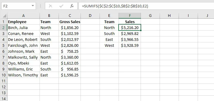
Note the use of absolute cell references above to lock the cell ranges. This prevents shifting of the range when the formula is copied to other cells.
5. COUNTIFS
The COUNTIFS function is another member of the IF family of functions. It counts only cells that satisfy all the stated criteria. COUNTIFS is superior to the COUNTIF function, which allows only one condition to be evaluated at a time.
The syntax of the COUNTIFS function is:
COUNTIFS(criteria_range1, criteria1, [criteria_range2, criteria2]…)
- Criteria_range1 - is the first range to be evaluated.
- Criteria1 - is the first criterion that cells in criteria_range1 must satisfy.
- Criteria_range2 - is the second range to be evaluated.
- Criteria2 - is the first criterion that cells in criteria_range2 must satisfy.
All pairs after criteria1 are optional. Up to 127 range and criteria pairs are allowed.
To count the number of sales reps on the North team who achieved more than $1,500 in sales, the formula would be:
=COUNTIFS(B2:B10,E1,C2:C10,E2)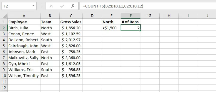 Note: In general, text values in COUNTIFS need to be enclosed in double quotes (""), and numbers do not. But when a logical operator (> or <) is used with a number, both the number and operator must be enclosed in quotation marks.
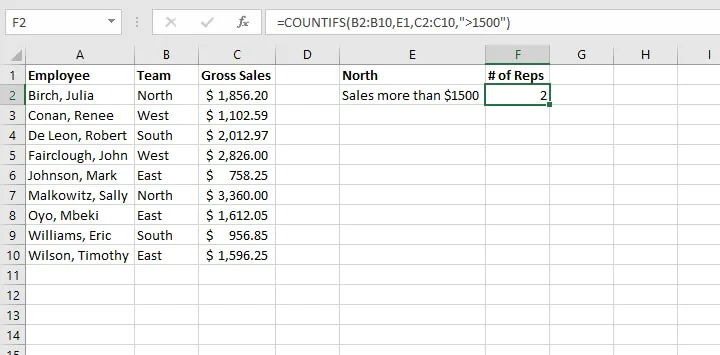
=COUNTIFS(B2:B10,E1,C2:C10,“>1500”)
6. VLOOKUP
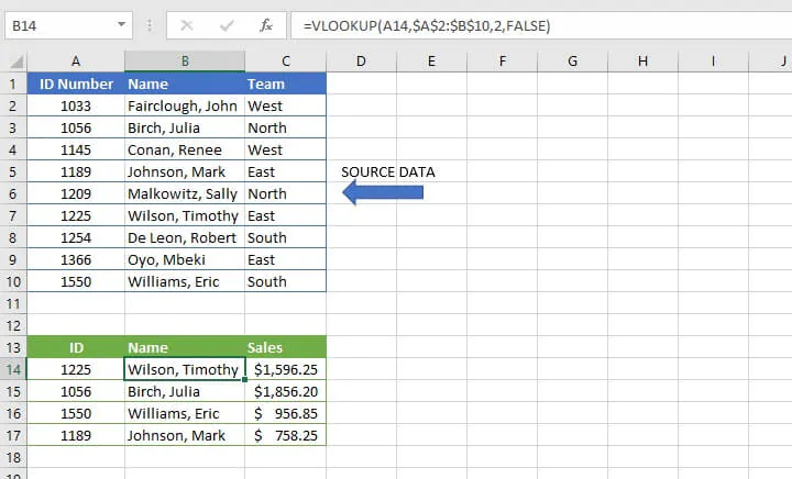
The VLOOKUP function will be a game-changer once you start using it. Use VLOOKUP when you need to find things in a table or an array. VLOOKUP is used in many search-type situations, for example, to find an employee name based on their employee ID.
The VLOOKUP syntax is:
VLOOKUP(lookup_value, table_array, col_index_num, [range_lookup])Here’s what those arguments mean:
- Lookup_value - is what you want to look up.
- Table_array - where you want to look for it.
- Col_index_num - is the column number in the range containing the value to return.
- Range_lookup - type TRUE for an approximate match, or FALSE for exact match.
The formula
=VLOOKUP(A14,$A$2:$B$10,2,FALSE)is entered in cell B14, which returns the name of the employee matching the ID number.
In recent years, VLOOKUP has been outperformed by XLOOKUP, which is more flexible and arguably easier to use. XLOOKUP is available in Microsoft 365 and later.
7. COUNT
The COUNT function will count the number of cells that contain numbers. You can use this function to get the number of entries in a number field that’s in a range or an array of numbers. The syntax of the COUNT function is:
=COUNT(value1, [value2]...)Placing the COUNT function in cell B6 below determines that there are three numeric values between cell B1 and B5.
=COUNT(B1:B5)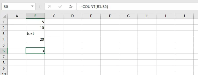
8. TRIM
The TRIM function will remove all spaces from text except for the single spaces between words. TRIM is often used on text imported from another application that may have irregular spacing.
Follow this simple format:
=TRIM(text)TRIM works on a text string entered within double quotes, or a single cell reference.
=TRIM(A1)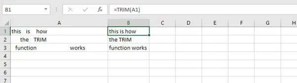
9. LEFT
The LEFT function is used to extract a specific number of characters from a text string, such as a specific portion of a telephone number. The syntax of the LEFT function is:
=LEFT(text, [num_chars])Num_chars refers to the number of characters to be extracted counting from the left. If the num_chars argument is omitted, Excel returns the leftmost character only.
=LEFT(A2,3)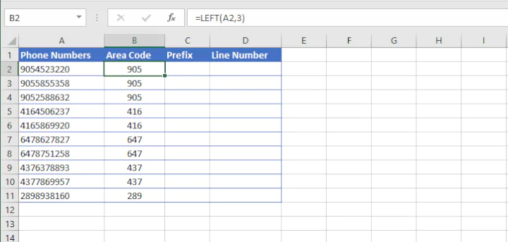
10. RIGHT
The RIGHT function is used to extract a specific number of characters from a text string, such as a specific portion of a telephone number. The syntax of the RIGHT function is:
=RIGHT(text, [num_chars])Num_chars refers to the number of characters to be extracted counting from the right. If the num_chars argument is omitted, Excel returns the rightmost character only.
=RIGHT(A2, 4)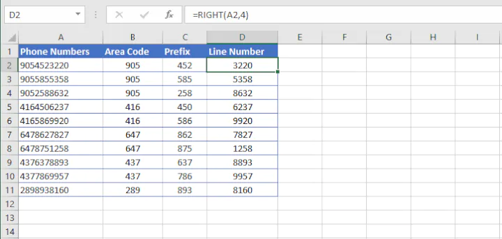
11. MID
The MID function is used to extract text from the middle of a text string. The syntax of the MID function is:
=MID(text, start_num, num_chars)The start_num argument tells Excel what position number to start extracting from (counting from the left), while num_chars tells it how many characters to extract.
=MID(A2,4,3)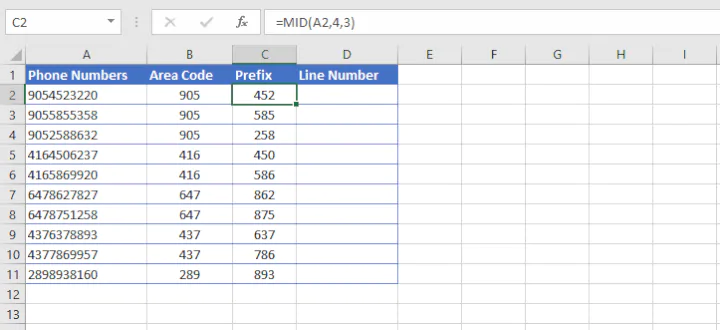
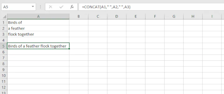
12. CONCAT
Our final basic Excel function is CONCAT. This function combines the values from multiple cells into one. This is useful for piecing together the different parts of text, for example, to combine a first name and last name into a full name. The syntax is:
=COUNT(text1, [text2], [text3]...)To insert delimiters (such as a space, dash, or comma) simply enter that bit of text as one of the text arguments within double quotes.
For example:
=CONCAT(A1," ",A2," ",A3)will copy the value from cells A2 and B2, inserting a space between them.
Conclusion - basic Excel formulas
And that's our top 12 Excel formulas list! Download the practice file and think about situations where you might use these functions at work.
- জুম আইটিতে ফিল্যান্সিং শিখুন- ভর্তি ফরম পূরন করতে ( এখানে ক্লিক করুন)

